42 pivot table 2 row labels

Pivot table row labels in separate columns • AuditExcel.co.za So when you click in the Pivot Table and click on the DESIGN tab one of the options is the Report Layout. Click on this and change it to Tabular form. Your pivot table report will now look like the bottom picture and will be easier to use in other areas of the spreadsheet and in our opinion is also easier to read. Pivot table on multiple consolidation ranges - 2 row labels Any idea how to display this particular kind of pivot table (ctrl+d, p) with two row labels? It's not as easy as in normal pivot table. I have only come up with a workaround, which is merging first two columns (=A1&"&"&B1) and using this combination as a row table, but it's nonsensical. Pivot table should be able to display two row labels.

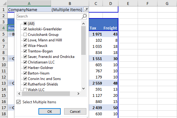
How to Filter Multiple Values in Pivot Table - Excel Tutorials Filter with Pivot Table Label Filters. Now we will clear all of our filters. To clear them all out at the same time, we will click anywhere on our Pivot Table, then go to PivotTable Analyze field >> Actions >> Clear Filters: Once we do that, we will go to our Pivot Table, go to a dropdown at the Row Labels >> Label Filters >> Contains:

Pivot table 2 row labels

Pivot Table adding "2" to value in answer set 1) Right click your pivot table -> Pivot table options -> Data -> Change "Number of items to retain per field" to NONE 2) Wipe all rows in your data source except for the headers 3) Refresh the pivot table 4) Save, and close all instances of Excel 5) Reopen the file, and paste your data 6) Refresh the pivot table Multi-level Pivot Table in Excel (In Easy Steps) Pivot table: 3. Next, click any cell inside the Sum of Amount2 column. 4. Right click and click on Value Field Settings. 5. Enter Percentage for Custom Name. 6. On the Show Values As tab, select % of Grand Total. 7. Click OK. Result: Multiple Report Filter Fields. First, insert a pivot table. Next, drag the following fields to the different areas. 1. Excel Pivot Table Row labels - Stack Overflow Right click on the pivot, go to PivotTable Options, Display Tab. Click on "Classic Pivot Table Layout" Go to each field (column), right click, field settings, layout & print tab. Click on "Repeat Item Labels" That should give you the table you're looking for. Share Improve this answer answered Nov 9, 2015 at 13:20 user1923975 1,359 3 13 28

Pivot table 2 row labels. Repeat item labels in a PivotTable Right-click the row or column label you want to repeat, and click Field Settings. Click the Layout & Print tab, and check the Repeat item labels box. Make sure Show item labels in tabular form is selected. Notes: When you edit any of the repeated labels, the changes you make are applied to all other cells with the same label. How to add side by side rows in excel pivot table ... First, you have to create a pivot table by choosing the rows, columns and values: Created pivot table should look like this: You have to right-click on pivot table and choose the PivotTable options. Then swich to Display tab and turn on Classic PivotTable layout: Now the pivot table should look like this: As a next step, you have to modify the Field settings of the rows: In subtotals section choose None: Use column labels from an Excel table as the rows in a ... I was able to do this using a combination of Excel's unpivot capability, combined with pivot tables. First, we can try unpivoting your data: Highlight your current table, including the headers; Then from the Data section of the ribbon, select From Table; Highlight all the columns containing data, but not the Year column, and then select Unpivot Columns How to Concatenate Values of Pivot Table | Basic Excel ... Click insert Pivot table, on the open window select the fields you want for your Pivot table. Once you select the desired fields, go to Analyze Menu. Under calculations, choose fields, Items & Sets tab then click on calculated fields. Enter the values and click ok. Your PivotTable will display the total of combined units and price.

Design the layout and format of a PivotTable Click anywhere in the PivotTable. This displays the PivotTable Tools tab on the ribbon. On the Options tab, in the PivotTable group, click Options. In the PivotTable Options dialog box, click the Layout & Format tab, and then under Layout, select or clear the Merge and center cells with labels check box. pivot table columns side by side - univcofc.org In pivot table I use Customer numbers as row labels and sales figures on Total Value. 0. 3: Click on any part of the data table. Find the Options button in the left side of the Analyze tab. Pivot table veterans remember the old Page area section of a pivot table. 4. 2. ". P.S. Step 4: Now let change Month as descending order on the left side ... How to Use Excel Pivot Table Label Filters The item is immediately hidden in the pivot table. Quickly Hide All But a Few Items. You can use a similar technique to hide most of the items in the Row Labels or Column Labels. Select the pivot table items that you want to keep visible; Right-click on one of the selected items; In the pop-up menu, click Filter, then click Keep Only Selected ... PDF Excel Troubleshooting Row Labels in Pivot Tables 2003 style of pivot table, where each row field gets its own column on the left side of the pivot table (see Figure 2). Filling in the Outline View in Excel 2010 A very common question is how to fill in the outline view in the left columns of a pivot table. For example, cells A5:A9 of Figure 2 should all say "Midwest." Cells B5:B9 should ...

How to Add Two-Tier Row Labels to the Pivot Table in ... Here are the steps to add the second-tier row label as the second column in the Pivot Table: Step 1: Click on any cell in the Pivot Table so that the Pivot table editor sidebar appears on the right side of Google... Step 2: Click Add button on the Rows header in the Pivot table editor sidebar. How to make row labels on same line in pivot table? 1. Click any one cell in the pivot table, and right click to choose PivotTable Options, see screenshot: 2. In the PivotTable Options dialog box, click the Display tab, and then check Classic PivotTable layout (enables... 3. Then click OK to close this dialog, and you will get the following pivot ... How to Customize Your Excel Pivot Chart Data Labels - dummies The Data Labels command on the Design tab's Add Chart Element menu in Excel allows you to label data markers with values from your pivot table. When you click the command button, Excel displays a menu with commands corresponding to locations for the data labels: None, Center, Left, Right, Above, and Below. None signifies that no data labels should be added to the chart and Show signifies ... Pivot table row labels side by side - Excel Tutorials Pivot table row labels side by side. Posted on October 29, 2018 July 20, 2020 by Tomasz ...

How to rename group or row labels in Excel PivotTable? 1. Click at the PivotTable, then click Analyze tab and go to the Active Field textbox. 2. Now in the Active Field textbox, the active field name is displayed, you can change it in the textbox. You can change other Row Labels name by clicking the relative fields in the PivotTable, then rename it in the Active Field textbox.

multiple fields as row labels on the same level in pivot ... multiple fields as row labels on the same level in pivot table Excel 2016. I am using Excel 2016. I have data that lists product models along with relevant data and also production volumes by month. Part of the relevant data are about 5 common part columns with the part # that applies to each model under the appropriate column.

How to Add Rows to a Pivot Table: 9 Steps (with Pictures) 3. Drag a field into the "Rows" area on PivotTable Fields. When you drag any of the fields in the upper portion of the PivotTable Fields panel to Rows, a new row will be added to your table. Rows are usually non-numeric fields, such as column headers. Numbers will usually go into the Values area. [1]

Pivot Table Multiple Row Labels? [SOLVED] You can, of course, create a pivot table that sums the values just at the owner level. then, create a second pivot table that sums the values at the Engineer level. If you need to present this data in a contiguous table, you can create a new Excel table and reference to the pivot table values with formulas (=PivotTableSheet!A1) cheers Microsoft MVP

Sort multiple row label in pivot table - Microsoft Community Sort multiple row label in pivot table. Could anybody suggest how to sort the pivot table row field data if it contains multiple headers :-. for example : In below given example I want to sort the data of column B in asending order , but when I am applying sorting here it is not sorting. Thanks in advance for your suggestion.

Pivot Table "Row Labels" Header Frustration - Microsoft ... Hi Everyone please help I can't change my headers from Row Labels in a Pivot Table. Using Excel 365

Share :