45 how to add custom data labels in excel
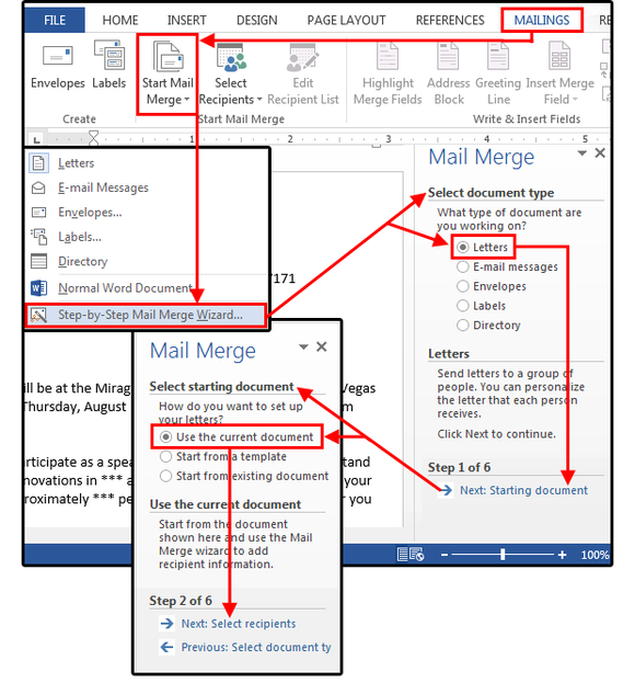
How to Add Axis Labels to a Chart in Excel | CustomGuide Add Data Labels. Use data labels to label the values of individual chart elements. Select the chart. Click the Chart Elements button. Click the Data Labels check box. In the Chart Elements menu, click the Data Labels list arrow to change the position of the data labels. How to Print Labels from Excel - Lifewire Select Mailings > Write & Insert Fields > Update Labels . Once you have the Excel spreadsheet and the Word document set up, you can merge the information and print your labels. Click Finish & Merge in the Finish group on the Mailings tab. Click Edit Individual Documents to preview how your printed labels will appear. Select All > OK .
Add data labels and callouts to charts in Excel 365 - EasyTweaks.com Step #1: After generating the chart in Excel, right-click anywhere within the chart and select Add labels . Note that you can also select the very handy option of Adding data Callouts. Step #2: When you select the "Add Labels" option, all the different portions of the chart will automatically take on the corresponding values in the table ...
How to add custom data labels in excel
Excel charts: add title, customize chart axis, legend and data labels Depending on where you want to focus your users' attention, you can add labels to one data series, all the series, or individual data points. Click the data series you want to label. To add a label to one data point, click that data point after selecting the series. Click the Chart Elements button, and select the Data Labels option. How to Change Excel Chart Data Labels to Custom Values? Now, click on any data label. This will select "all" data labels. Now click once again. At this point excel will select only one data label. Go to Formula bar, press = and point to the cell where the data label for that chart data point is defined. Repeat the process for all other data labels, one after another. See the screencast. Excel tutorial: How to customize axis labels Instead you'll need to open up the Select Data window. Here you'll see the horizontal axis labels listed on the right. Click the edit button to access the label range. It's not obvious, but you can type arbitrary labels separated with commas in this field. So I can just enter A through F. When I click OK, the chart is updated.
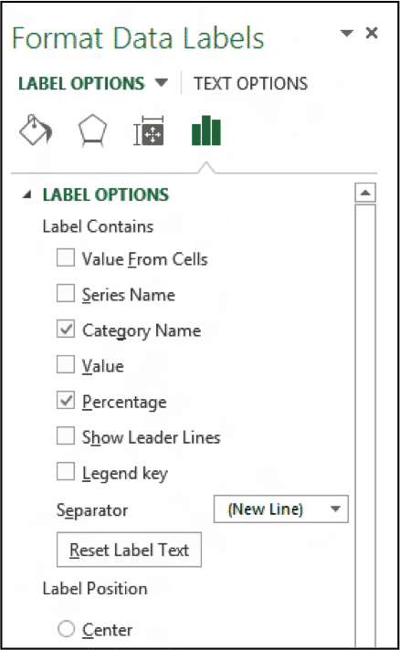
How to add custom data labels in excel. Custom Axis Labels and Gridlines in an Excel Chart In Excel 2007-2010, go to the Chart Tools > Layout tab > Data Labels > More Data Label Options. In Excel 2013, click the "+" icon to the top right of the chart, click the right arrow next to Data Labels, and choose More Options…. Then in either case, choose the Label Contains option for X Values and the Label Position option for Below. How to add and customize chart data labels - Get Digital Help Double press with left mouse button on with left mouse button on a data label series to open the settings pane. Go to tab "Label Options" see image to the right. This setting allows you to change the number formatting of the data labels. The image below shows numbers formatted as dates. How to Create Labels in Word from an Excel Spreadsheet In this guide, you'll learn how to create a label spreadsheet in Excel that's compatible with Word, configure your labels, and save or print them. Table of Contents 1. Enter the Data for Your Labels in an Excel Spreadsheet 2. Configure Labels in Word 3. Bring the Excel Data Into the Word Document 4. Add Labels from Excel to a Word Document 5. Edit titles or data labels in a chart - support.microsoft.com The first click selects the data labels for the whole data series, and the second click selects the individual data label. Right-click the data label, and then click Format Data Label or Format Data Labels. Click Label Options if it's not selected, and then select the Reset Label Text check box. Top of Page
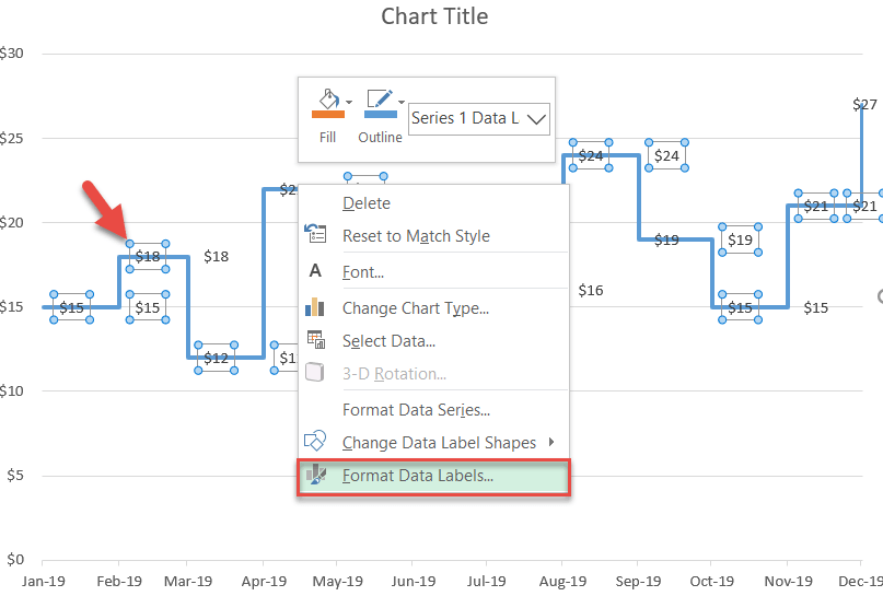
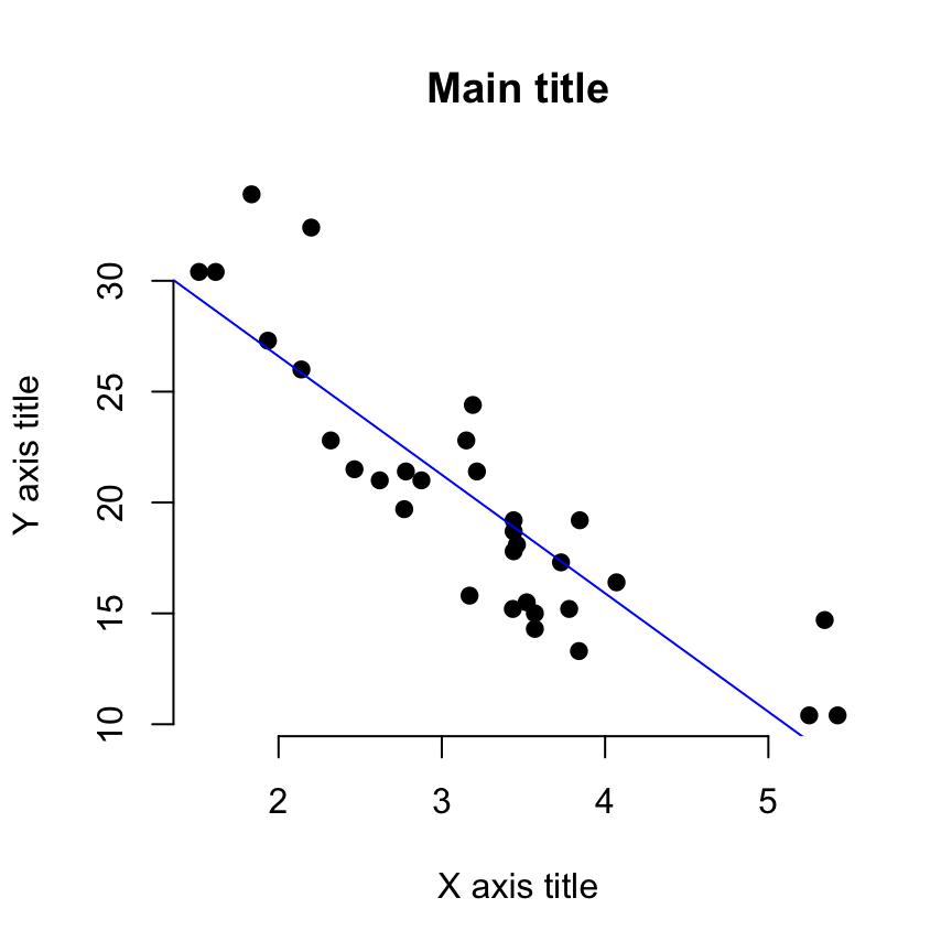
Custom Y-Axis Labels in Excel - PolicyViz 1. Select that column and change it to a scatterplot. 2. Select the point, right-click to Format Data Series and plot the series on the Secondary Axis. 3. Show the Secondary Horizontal axis by going to the Axes menu under the Chart Layout button in the ribbon. (Notice how the point moves over when you do so.) 4. How to Add Data Labels to an Excel 2010 Chart - dummies On the Chart Tools Layout tab, click Data Labels→More Data Label Options. The Format Data Labels dialog box appears. You can use the options on the Label Options, Number, Fill, Border Color, Border Styles, Shadow, Glow and Soft Edges, 3-D Format, and Alignment tabs to customize the appearance and position of the data labels. Add or remove data labels in a chart - support.microsoft.com To label one data point, after clicking the series, click that data point. In the upper right corner, next to the chart, click Add Chart Element > Data Labels. To change the location, click the arrow, and choose an option. If you want to show your data label inside a text bubble shape, click Data Callout. How to Customize Your Excel Pivot Chart Data Labels To add data labels, just select the command that corresponds to the location you want. To remove the labels, select the None command. If you want to specify what Excel should use for the data label, choose the More Data Labels Options command from the Data Labels menu. Excel displays the Format Data Labels pane.
Add Custom Labels to x-y Scatter plot in Excel Step 1: Select the Data, INSERT -> Recommended Charts -> Scatter chart (3 rd chart will be scatter chart) Let the plotted scatter chart be Step 2: Click the + symbol and add data labels by clicking it as shown below Step 3: Now we need to add the flavor names to the label. Now right click on the label and click format data labels. Using the CONCAT function to create custom data labels for an Excel ... Adding the custom labels to the data series You can create the standard line graph by selecting the data in cells A4 to B16 and creating a line graph. Notice that we do not select the custom label column when selecting the data to create the graph. Format the graph as you want (here are tips on making it professional looking ). How to create Custom Data Labels in Excel Charts Add default data labels; Click on each unwanted label (using slow double click) and delete it; Select each item where you want the custom label one at a time; Press F2 to move focus to the Formula editing box; Type the equal to sign; Now click on the cell which contains the appropriate label; Press ENTER; That's it. Now that data label is linked to that cell. How to add data labels from different column in an Excel chart? This method will guide you to manually add a data label from a cell of different column at a time in an Excel chart. 1. Right click the data series in the chart, and select Add Data Labels > Add Data Labels from the context menu to add data labels. 2. Click any data label to select all data labels, and then click the specified data label to select it only in the chart.
Mail Merge master class: How to merge your Excel contact database with custom letters in Word ...
Apply Custom Data Labels to Charted Points - Peltier Tech Click once on a label to select the series of labels. Click again on a label to select just that specific label. Double click on the label to highlight the text of the label, or just click once to insert the cursor into the existing text. Type the text you want to display in the label, and press the Enter key.

35 Data Label Excel - Labels For Your Ideas
Add a DATA LABEL to ONE POINT on a chart in Excel Click on the chart line to add the data point to. All the data points will be highlighted. Click again on the single point that you want to add a data label to. Right-click and select ' Add data label ' This is the key step! Right-click again on the data point itself (not the label) and select ' Format data label '.
How to Create a Step Chart in Excel - Automate Excel
Custom data labels in a chart - Get Digital Help If you have excel 2013 you can use custom data labels on a scatter chart. 1. Right press with mouse on a series 2. Press with left mouse button on "Add Data Labels" 3. Right press with mouse again on a series 4. Press with left mouse button on "Format Data Labels" 5. Enable check box "Value from cells" 6. Select a cell range 7. Disable check box "Y Value"
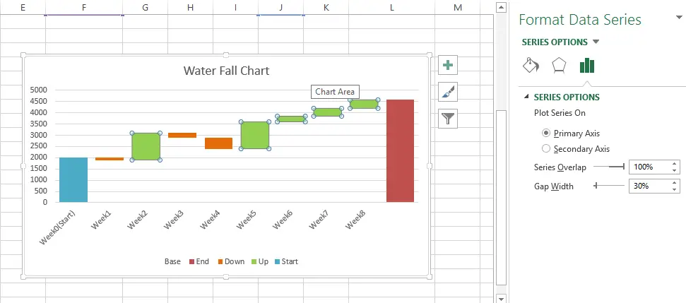
Waterfall Chart in Excel - DataScience Made Simple
Custom Chart Data Labels In Excel With Formulas Follow the steps below to create the custom data labels. Select the chart label you want to change. In the formula-bar hit = (equals), select the cell reference containing your chart label's data. In this case, the first label is in cell E2. Finally, repeat for all your chart laebls.
![Custom Data Labels with Colors and Symbols in Excel Charts - [How To] - PakAccountants.com](http://pakaccountants.com/wp-content/uploads/2014/09/data-label-chart-6.gif)
Custom Data Labels with Colors and Symbols in Excel Charts - [How To] - PakAccountants.com
How to add or move data labels in Excel chart? - ExtendOffice In Excel 2013 or 2016. 1. Click the chart to show the Chart Elements button . 2. Then click the Chart Elements, and check Data Labels, then you can click the arrow to choose an option about the data labels in the sub menu. See screenshot:
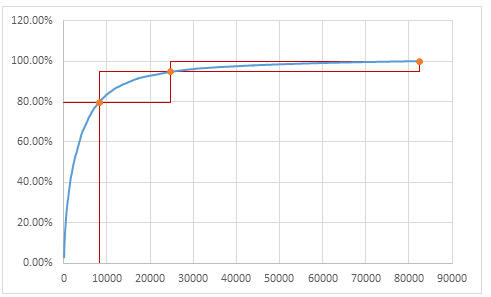
ABC Inventory Analysis - Tutorial & Excel Template | Chandoo.org - Learn Microsoft Excel Online
Excel tutorial: How to use data labels In this video, we'll cover the basics of data labels. Data labels are used to display source data in a chart directly. They normally come from the source data, but they can include other values as well, as we'll see in in a moment. Generally, the easiest way to show data labels to use the chart elements menu. When you check the box, you'll see ...

Enable or Disable Excel Data Labels at the click of a button - How To - PakAccountants.com
Format Data Labels in Excel- Instructions - TeachUcomp, Inc. To do this, click the "Format" tab within the "Chart Tools" contextual tab in the Ribbon. Then select the data labels to format from the "Chart Elements" drop-down in the "Current Selection" button group. Then click the "Format Selection" button that appears below the drop-down menu in the same area.

Enable or Disable Excel Data Labels at the click of a button - How To - PakAccountants.com
Custom Data Labels with Colors and Symbols in Excel Charts - [How To] Step 2: Left click on any data label and it will select all of them or at least all the data labels of that series. Left click again and this time only the data label you clicked will be selected. Step 3: Click inside the formula bar, Hit "=" button on keyboard and then click on the cell you want to link or type the address of that cell.

E-xcel Tuts: Add Data Labels to Excel Charts
Adding rich data labels to charts in Excel 2013 | Microsoft 365 Blog To add a data label in a shape, select the data point of interest, then right-click it to pull up the context menu. Click Add Data Label, then click Add Data Callout . The result is that your data label will appear in a graphical callout. In this case, the category Thr for the particular data label is automatically added to the callout too.

Excel tutorial: How to customize axis labels Instead you'll need to open up the Select Data window. Here you'll see the horizontal axis labels listed on the right. Click the edit button to access the label range. It's not obvious, but you can type arbitrary labels separated with commas in this field. So I can just enter A through F. When I click OK, the chart is updated.
31 Label Scatter Plot Excel - Label Design Ideas 2020
How to Change Excel Chart Data Labels to Custom Values? Now, click on any data label. This will select "all" data labels. Now click once again. At this point excel will select only one data label. Go to Formula bar, press = and point to the cell where the data label for that chart data point is defined. Repeat the process for all other data labels, one after another. See the screencast.
Format Data Labels in Excel 2013- Tutorial - TeachUcomp, Inc.
Excel charts: add title, customize chart axis, legend and data labels Depending on where you want to focus your users' attention, you can add labels to one data series, all the series, or individual data points. Click the data series you want to label. To add a label to one data point, click that data point after selecting the series. Click the Chart Elements button, and select the Data Labels option.
How to Import Excel Data into a Label File in Text Labels | Brady Support

How to create Custom Data Labels in Excel Charts - Efficiency 365
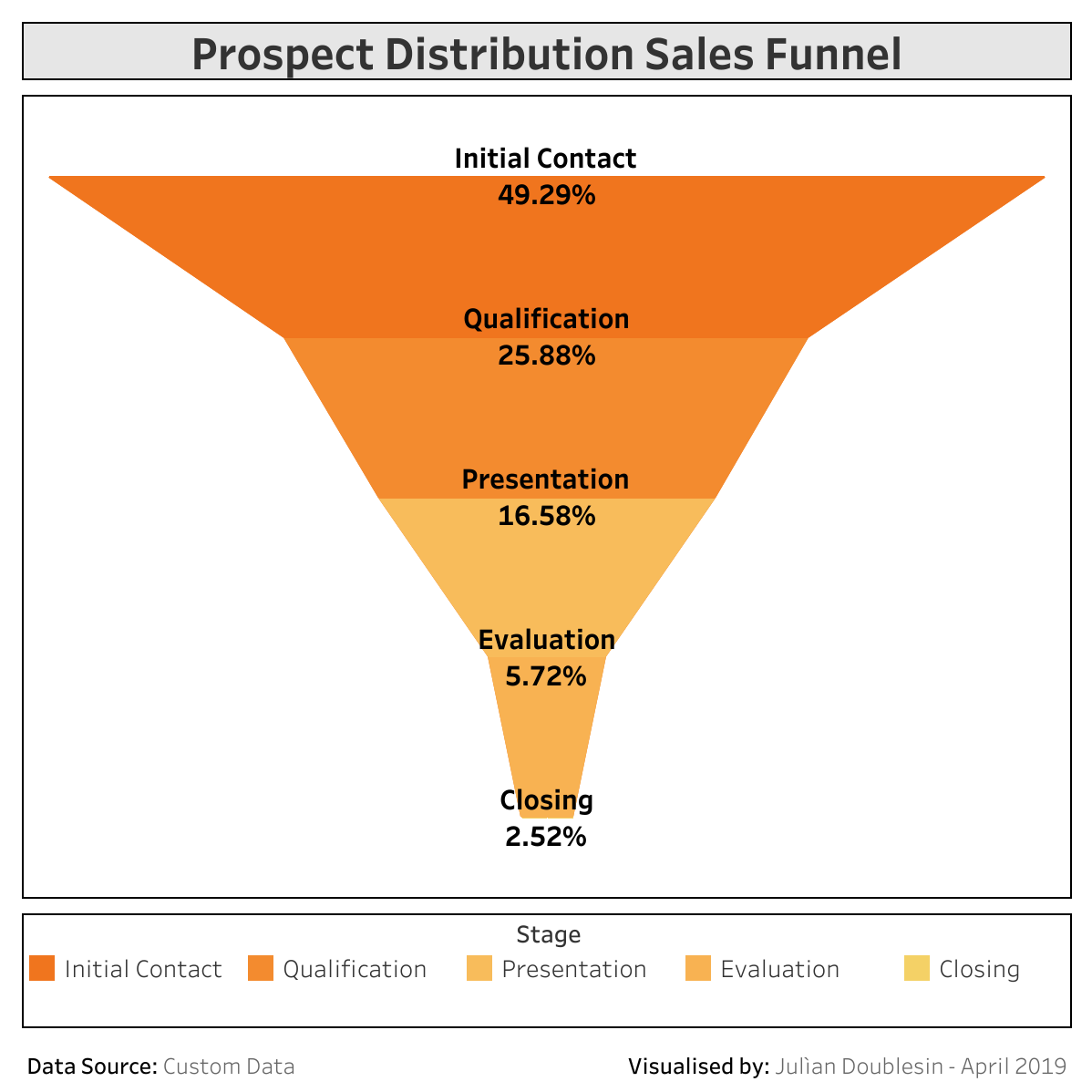
Tableau: Custom Shape Series: The Funnel Chart | by Julian Doublesin | Medium
Excel Tips - How to show custom data labels in charts - YouTube
Chart axes, legend, data labels, trendline in Excel - Tech Funda
Post a Comment for "45 how to add custom data labels in excel"