41 data labels excel 2013

Add a Data Callout Label to Charts in Excel 2013 Dec 09, 2013 · The new Data Callout Labels make it easier to show the details about the data series or its individual data points in a clear and easy to read format. How to Add a Data Callout Label. Click on the data series or chart. In the upper right corner, next to your chart, click the Chart Elements button (plus sign), and then click Data Labels. Values From Cell: Missing Data Labels Option in Excel 2013? 8. May 27, 2015. #1. Ive inherited a Powerpoin with an embedded Excel chart and data sheet. The graph in Powerpoint shows several instances of a value [CellRange]. Im trying to figure out where its "trying" to pull its data from and I think because the data is not in a contiguous range its having trouble. A couple articles refer to formatting ...

support.microsoft.com › en-us › officeTutorial: Import Data into Excel, and Create a Data Model In the next tutorial, Extend Data Model relationships using Excel 2013, Power Pivot, and DAX, you build on what you learned here, and step through extending the Data Model using a powerful and visual Excel add-in called Power Pivot. You also learn how to calculate columns in a table, and use that calculated column so that an otherwise unrelated ...

Data labels excel 2013

Edit titles or data labels in a chart - support.microsoft.com You can also place data labels in a standard position relative to their data markers. Depending on the chart type, you can choose from a variety of positioning options. On a chart, do one of the following: To reposition all data labels for an entire data series, click a data label once to select the data series. Tip - Adding rich data labels to charts in Excel 2013 You can do this by adjusting the zoom control on the bottom right corner of Excel's chrome. Then, select the value in the data label and hit the right-arrow key on your keyboard. The story behind the data in our example is that the temperature increased significantly on Wednesday and that appeared to help drive up business at the lemonade stand. Change the format of data labels in a chart To get there, after adding your data labels, select the data label to format, and then click Chart Elements > Data Labels > More Options. To go to the appropriate area, click one of the four icons ( Fill & Line, Effects, Size & Properties ( Layout & Properties in Outlook or Word), or Label Options) shown here.

Data labels excel 2013. Tutorial: Import Data into Excel, and Create a Data Model Import Data into Excel 2013, and Create a Data Model. Extend Data Model relationships using Excel, Power Pivot, and DAX. ... Fencing, Figure Skating, and Speed Skating. You can do this from within the PivotTable Fields area, or from the Row Labels filter in the PivotTable itself. Click anywhere in the PivotTable to ensure the Excel PivotTable ... mgconsulting.wordpress.com › 2013/12/09 › add-a-dataAdd a Data Callout Label to Charts in Excel 2013 Dec 09, 2013 · The new Data Callout Labels make it easier to show the details about the data series or its individual data points in a clear and easy to read format. How to Add a Data Callout Label. Click on the data series or chart. In the upper right corner, next to your chart, click the Chart Elements button (plus sign), and then click Data Labels. How to Change Excel Chart Data Labels to Custom Values? May 05, 2010 · Now, click on any data label. This will select “all” data labels. Now click once again. At this point excel will select only one data label. Go to Formula bar, press = and point to the cell where the data label for that chart data point is defined. Repeat the process for all other data labels, one after another. See the screencast. Values From Cell: Missing Data Labels Option in Excel 2013? When a chart created in 2013 using the "Values from Cell" data label option is opened with any earlier version of Excel, the data labels will show as " [CELLRANGE]". If you want to ensure that data labels survive different generations of Excel, you need to revert to the old technique: Insert data labels Edit each individual data label

Add or remove data labels in a chart - support.microsoft.com Right-click the data series or data label to display more data for, and then click Format Data Labels. Click Label Options and under Label Contains, select the Values From Cells checkbox. When the Data Label Range dialog box appears, go back to the spreadsheet and select the range for which you want the cell values to display as data labels. How to add data labels from different column in an Excel chart? Right click the data series in the chart, and select Add Data Labels > Add Data Labels from the context menu to add data labels. 2. Click any data label to select all data labels, and then click the specified data label to select it only in the chart. 3. Make and print Excel labels from worksheet data - Ablebits Get address and mailing labels for printing The tool will create a copy of your table with a transformed layout, so you can easily print your data.; Choose to place the labels in two or more columns Enter the number of columns you want to see on the resulting worksheet.; Separate the cards by a blank row or column Add an empty row and column between the labels for … formatting - How to format Microsoft Excel data labels without trailing ... To get this to work, I formatted the cell's of the data column 4 4 4 4 3.5 13.5, by either selecting the column and then right click and format cells or by right clicking on the chart and selecting format data labels.I formatted this with the regular expression $#K so that the data then shows as $4K $4K $4K $4K $4K $14K. The consequence is that the number is rounded to not include the decimal.

Quick Tip: Excel 2013 offers flexible data labels | TechRepublic right-click and choose Insert Data Label Field. In the next dialog, select [Cell] Choose Cell. When Excel displays the source dialog, click the cell that contains the MIN () function, and click OK.... › format-data-labels-in-excelFormat Data Labels in Excel- Instructions - TeachUcomp, Inc. Nov 14, 2019 · Then select the “Format Data Labels…” command from the pop-up menu that appears to format data labels in Excel. Using either method then displays the “Format Data Labels” task pane at the right side of the screen. Format Data Labels in Excel- Instructions: A picture of the “Format Data Labels” task pane in Excel. How to add or move data labels in Excel chart? - ExtendOffice To add or move data labels in a chart, you can do as below steps: In Excel 2013 or 2016. 1. Click the chart to show the Chart Elements button .. 2. Then click the Chart Elements, and check Data Labels, then you can click the arrow to choose an option about the data labels in the sub menu.See screenshot: › excel › how-to-add-total-dataHow to Add Total Data Labels to the Excel Stacked Bar Chart Apr 03, 2013 · Step 4: Right click your new line chart and select “Add Data Labels” Step 5: Right click your new data labels and format them so that their label position is “Above”; also make the labels bold and increase the font size. Step 6: Right click the line, select “Format Data Series”; in the Line Color menu, select “No line”

M. Barros (in English): Sampling without replacement in Excel

› charts › dynamic-chart-dataCreate Dynamic Chart Data Labels with Slicers - Excel Campus Feb 10, 2016 · Typically a chart will display data labels based on the underlying source data for the chart. In Excel 2013 a new feature called “Value from Cells” was introduced. This feature allows us to specify the a range that we want to use for the labels. Since our data labels will change between a currency ($) and percentage (%) formats, we need a ...

Surface Chart in Excel

Excel Tips n Tricks -Tip 8 (Applying Chart Data Labels From a Range in ... Click on the plus symbol, the first icon, and check "Data Labels". Now you will see them added to your chart. You can also click on the right arrow on "Data Labels" and select where you want the data labels to be aligned, in other words center, right, top, bottom and so on. Picture 4 4. I modified the chart and axis titles to look good.

FORMS FOR FREE: M1a Member Data Record

Creating a chart with dynamic labels - Microsoft Excel 2013 Excel 2013 365 2016. This tip shows how to create dynamically updated chart labels that depend on value or other cells. ... For all labels: on the Format Data Labels task pane, in the Label Options, in the Label Contains group, check Value From Cells and then choose cells:

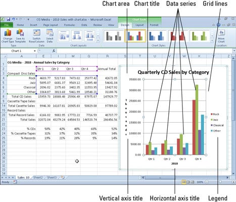
Getting to Know the Parts of an Excel 2010 Chart - dummies

How to Customize Chart Elements in Excel 2013 - dummies To add data labels to your selected chart and position them, click the Chart Elements button next to the chart and then select the Data Labels check box before you select one of the following options on its continuation menu: Center to position the data labels in the middle of each data point. Inside End to position the data labels inside each ...

Integrating Technology in the Elementary Classroom: Creating A Drop Down Box in Excel

Format Data Labels in Excel- Instructions - TeachUcomp, Inc. Nov 14, 2019 · Then select the “Format Data Labels…” command from the pop-up menu that appears to format data labels in Excel. Using either method then displays the “Format Data Labels” task pane at the right side of the screen. Format Data Labels in Excel- Instructions: A picture of the “Format Data Labels” task pane in Excel.

Share :