45 multiple data labels excel pie chart
Solved: Show multiple data lables on a chart - Power BI 09-07-2017 06:25 AM Is there a way to display multiple labels on a chart? For example, I'd like to include both the total and the percent on pie chart. Or instead of having a separate legend include the series name along with the % in a pie chart. I know they can be viewed as tool tips, but this is not sufficient for my needs. How to add data labels from different column in an Excel ... This method will introduce a solution to add all data labels from a different column in an Excel chart at the same time. Please do as follows: 1. Right click the data series in the chart, and select Add Data Labels > Add Data Labels from the context menu to add data labels. 2.
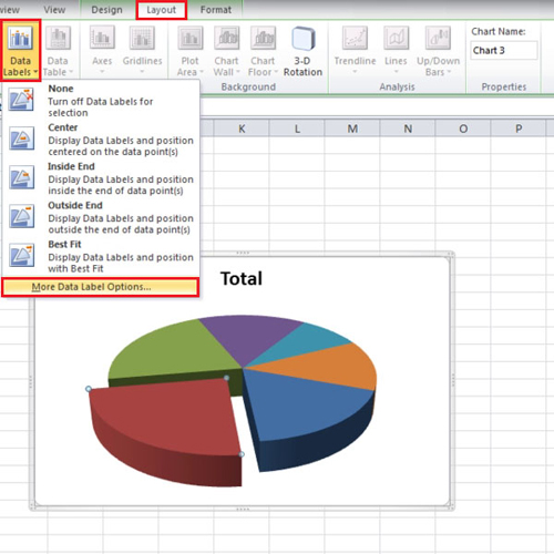
Add or remove data labels in a chart Click the data series or chart. To label one data point, after clicking the series, click that data point. In the upper right corner, next to the chart, click Add Chart Element > Data Labels. To change the location, click the arrow, and choose an option. If you want to show your data label inside a text bubble shape, click Data Callout.

Multiple data labels excel pie chart
How to create a Multiple Pies charts - Datawrapper Academy The most important thing you have to keep in mind is that a pie chart always represents a whole, i.e. 100%. Therefore, you can only use data that is based on exclusive values. Making a pie chart of a survey that allows multiple answers will lead to a misleading chart. Use a bar chart instead, but never a pie chart. Connecting Pie Chart Copies Across Multiple Sheets ... Connecting Pie Chart Copies Across Multiple Sheets I have a large spreadsheet where I'm both working with raw data and creating display pages for my co-workers to view. I have one mastersheet where I have all the pie charts I created from different pivot tables. Create a multi-level category chart in Excel - ExtendOffice 2. Select the data range, click Insert > Insert Column or Bar Chart > Clustered Bar.. 3. Drag the chart border to enlarge the chart area. See the below demo. 4. Right click the bar and select Format Data Series from the right-clicking menu to open the Format Data Series pane.. Tips: You can also double click any of the bars to open the Format Data Series pane.
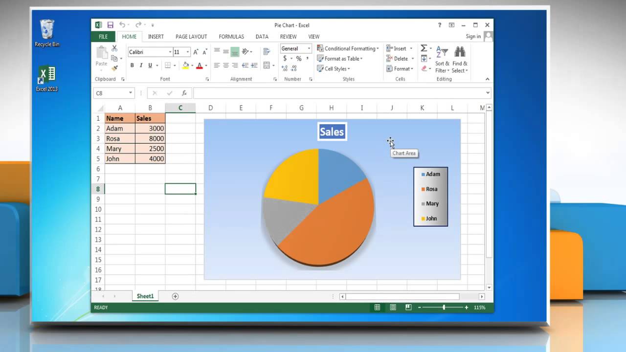
Multiple data labels excel pie chart. How to Create Pie Charts in Excel (In Easy Steps) 6. Create the pie chart (repeat steps 2-3). 7. Click the legend at the bottom and press Delete. 8. Select the pie chart. 9. Click the + button on the right side of the chart and click the check box next to Data Labels. 10. Click the paintbrush icon on the right side of the chart and change the color scheme of the pie chart. Result: 11. Adding data labels to a pie chart - Excel General - OzGrid ... But it didn't record anything about labels, much less making them bold. In fact, I tried recording multiple macros (create the chart from scratch, modify a created chart, etc.) and still nothing about labels. The macros I recorded without touching the labels look the same as the ones with. Do you know why that is? Thanks a lot. How to Create Multi-Category Charts in Excel ... Step 1: Insert the data into the cells in Excel. Now select all the data by dragging and then go to "Insert" and select "Insert Column or Bar Chart". A pop-down menu having 2-D and 3-D bars will occur and select "vertical bar" from it. Select the cell -> Insert -> Chart Groups -> 2-D Column Bar Chart Insertion Multi-Category Chart Excel Pie Chart Multiple Labels Quickly create multiple progress pie charts in one graph. Excel Details: 1.Click Kutools > Charts > Difference Comparison > Progress Pie Chart to go to the Progress Pie Chart dialog box. 2. In the popped out dialog box, select the data range of the axis labels, actual values and target values under the Axis Labels, Actual Value and Target Value boxes separately.
Everything You Need to Know About Pie Chart in Excel How to Make a Pie Chart in Excel. Start with selecting your data in Excel. If you include data labels in your selection, Excel will automatically assign them to each column and generate the chart. Go to the INSERT tab in the Ribbon and click on the Pie Chart icon to see the pie chart types. Click on the desired chart to insert. Pie of Pie Chart in Excel - Inserting, Customizing - Excel ... Customizing the Pie of Pie Chart in Excel Splitting the Parent Chart We can select what slices are going to be represented by the parent chart and subset chart. To begin:- Select the Chart. Go to Format Tab. Choose Series "Sales" in the Current Selection Group. Click on Format Selection Button. This would again open Format Series pane. Pie Chart in Excel | How to Create Pie Chart | Step-by ... Pie Chart in Excel is used for showing the completion or main contribution of different segments out of 100%. It is like each value represents the portion of the Slice from the total complete Pie. For Example, we have 4 values A, B, C and D. Solved: Pie chart showing duplicates - Power Platform ... Pie chart showing duplicates. 12-15-2019 07:21 AM. I have been working on a pie chart in my app that is being used as a time keeper for company projects, and it is quickly becoming the bane of my existence. I have a drop down that when you select a person's name, it pulls up a pie chart with all of the projects they have worked on and the time ...
Create Multiple Pie Charts in Excel using Worksheet Data ... HasDataLabels = True End With ' SET NEW LOCATION FOR THE NEW CHART (CALCULATED BASED OF CHART WIDTH). ileft = ileft + 200 Next i End Sub Now, just click the button and it will automatically add Multiple Pie Charts below the data (on the same sheet), along with Data Labels over each slice of the chart. How to fix wrapped data labels in a pie chart | Sage ... 1. Right click on the data label and select Format Data Labels 2. Select Text Options > Text Box > and un-select Wrap text in shape. 3. The data labels resize to fit all the text on one line. 4. Alternatively, by double-clicking a data label, the handles can be used to resize the label to wrap words as desired. How to Make a Pie Chart in Excel (Only Guide You Need ... To do this select the More Options from Data labels under the Chart Elements or by selecting the chart right click on to the mouse button and select Format Data Labels. This will open up the Format Data Label option on the right side of your worksheet. Click on the percentage. If you want the value with the percentage click on both and close it. How to Combine or Group Pie Charts in Microsoft Excel Click on the first chart and then hold the Ctrl key as you click on each of the other charts to select them all. Click Format > Group > Group. All pie charts are now combined as one figure. They will move and resize as one image. Choose Different Charts to View your Data
Excel VBA Codes & Macros: Hide all data label less than any percentage in Pie Chart Using VBA
How to Show Percentage in Pie Chart in Excel? - GeeksforGeeks The steps are as follows : Select the pie chart. Right-click on it. A pop-down menu will appear. Click on the Format Data Labels option. The Format Data Labels dialog box will appear. In this dialog box check the "Percentage" button and uncheck the Value button. This will replace the data labels in pie chart from values to percentage.
How to Make a Pie Chart in Excel & Add Rich Data Labels to The Chart!
Edit titles or data labels in a chart - support.microsoft.com The first click selects the data labels for the whole data series, and the second click selects the individual data label. Right-click the data label, and then click Format Data Label or Format Data Labels. Click Label Options if it's not selected, and then select the Reset Label Text check box. Top of Page
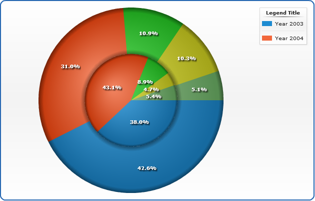
Pie and Donut Chart
Multiple data labels (in separate locations on chart) Re: Multiple data labels (in separate locations on chart) You can do it in a single chart. Create the chart so it has 2 columns of data. At first only the 1 column of data will be displayed. Move that series to the secondary axis. You can now apply different data labels to each series. Attached Files 819208.xlsx (13.8 KB, 263 views) Download

How to Make a Pie Chart in Excel & Add Rich Data Labels to The Chart!
Pie Chart with percent data on multiple columns - Power BI If you do not want to break the initial table, you can use union () function to create a new calculate table: Rename the column as 'Type', create a pie chart to get the result: If this post helps then please consider Accept it as the solution to help the other members find it more quickly. 06-22-2020 07:17 AM.

How to Make a Pie Chart in Excel & Add Rich Data Labels to The Chart!
Doughnut Chart in Excel | How to Create Doughnut Chart in ... Click on the Insert menu. Go to charts select the PIE chart drop-down menu. From Dropdown, select the doughnut symbol. Then the below chart will appear on the screen with two doughnut rings. To reduce the doughnuts hole size, select the doughnuts and right-click and then select Format data series.

Quickly Create A Year Over Year Comparison Bar Chart In Excel
Pie Chart in Excel - Inserting, Formatting, Filters, Data ... Right click on the Data Labels on the chart. Click on Format Data Labels option. Consequently, this will open up the Format Data Labels pane on the right of the excel worksheet. Mark the Category Name, Percentage and Legend Key. Also mark the labels position at Outside End. This is how the chark looks. Formatting the Chart Background, Chart Styles

Advanced Graphs Using Excel : Gantt Chart in Excel - plot your calender activities
Multiple Data Labels on a Pie Chart | MrExcel Message Board So I have a table with 8 rows and 3 columns. This table includes: Column 1 - shipment name Column 2 - shipment cost Column 3 - shipment weight I have created a pie chart from this table, which covers the first two columns. Displayed next to each slice is a label with the shipment name, shipment cost, and percent share of the pie.

How to Create Multi-Category Chart in Excel - Excel Board
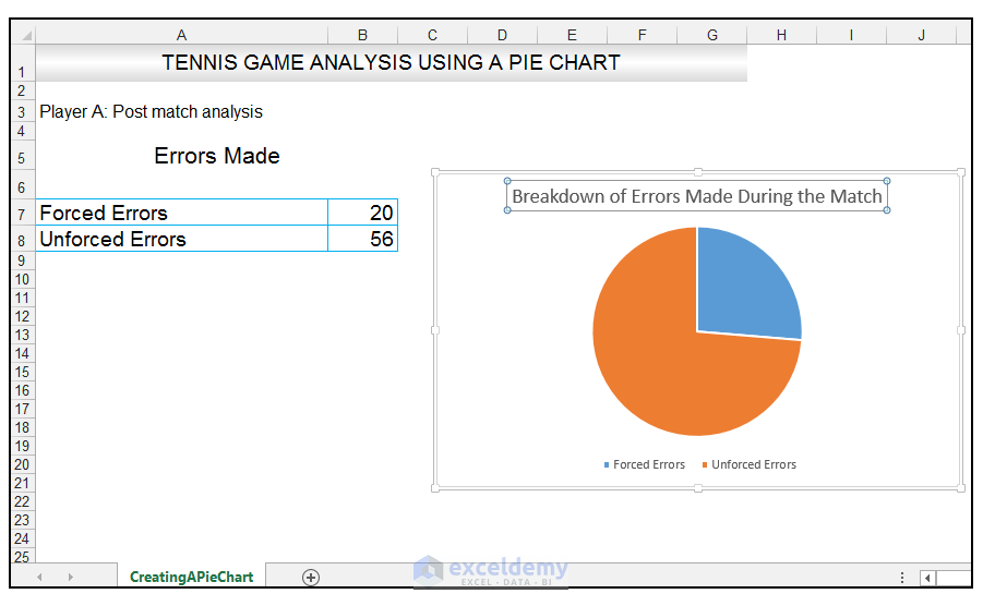
Creating Pie Chart and Adding/Formatting Data Labels (Excel) Creating Pie Chart and Adding/Formatting Data Labels (Excel)
How to Create and modify a pie chart in Excel | HowTech
How to Create a Pie Chart in Excel | Smartsheet To create a pie chart in Excel 2016, add your data set to a worksheet and highlight it. Then click the Insert tab, and click the dropdown menu next to the image of a pie chart. Select the chart type you want to use and the chosen chart will appear on the worksheet with the data you selected.
How to insert data labels in a Pie chart in Excel 2013 - YouTube
How to create a pie chart with multiple data series - Quora Answer (1 of 5): Please don't. Pie charts are never the right way to represent data, and the problems associated with them only get worse when you're trying to compare multiple sets of data. It's very difficult to make area comparisons by eye (which is essentially how a pie chart is representing ...
How do I change the order of pie chart slices?
Create a multi-level category chart in Excel - ExtendOffice 2. Select the data range, click Insert > Insert Column or Bar Chart > Clustered Bar.. 3. Drag the chart border to enlarge the chart area. See the below demo. 4. Right click the bar and select Format Data Series from the right-clicking menu to open the Format Data Series pane.. Tips: You can also double click any of the bars to open the Format Data Series pane.
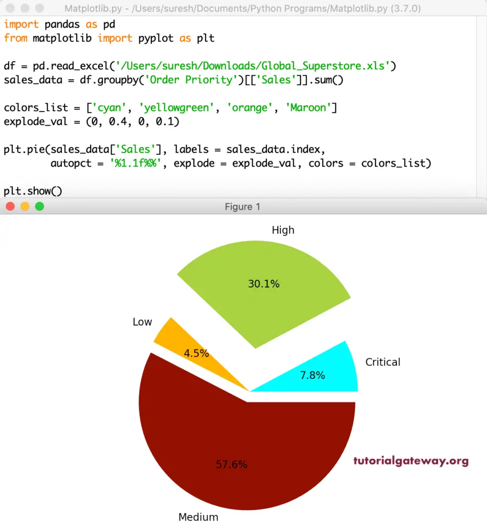
Python matplotlib Pie Chart
Connecting Pie Chart Copies Across Multiple Sheets ... Connecting Pie Chart Copies Across Multiple Sheets I have a large spreadsheet where I'm both working with raw data and creating display pages for my co-workers to view. I have one mastersheet where I have all the pie charts I created from different pivot tables.
How to Make a Pie Chart in Excel & Add Rich Data Labels to The Chart!
How to create a Multiple Pies charts - Datawrapper Academy The most important thing you have to keep in mind is that a pie chart always represents a whole, i.e. 100%. Therefore, you can only use data that is based on exclusive values. Making a pie chart of a survey that allows multiple answers will lead to a misleading chart. Use a bar chart instead, but never a pie chart.

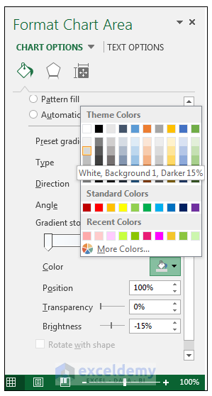
Change color of data label placed, using the 'best fit' option, outside a pie chart - Excel 2010 ...

vba - Pie Chart - Move Data Labels off Chart - Stack Overflow
Post a Comment for "45 multiple data labels excel pie chart"