40 how to add data labels to a pie chart in excel
Pie of Pie Chart in Excel - Inserting, Customizing - Excel ... 03/01/2022 · In the above example, there were a total of 6 data points. The Parent Pie chart represents three of them i.e Facebook, Youtube, and Instagram while the fourth data point named “Other” splits into a subset Pie chart that represents the rest of the three data points i.e Zee, Linkedin, and Hotstar. Waterfall Chart in Excel (Examples) | How to ... - EDUCBA Select the blue bricks and right-click and select the option ”Add Data Labels”. Then you will get the values on the bricks; for better visibility, change the brick color to light blue. Double click on the “chart title” and change to the waterfall chart. If you observe, we can see both monthly sales and accumulated sales in the singles chart. The values in each brick represent the ...
How do you make a pie chart on a laptop? | Blog Manually add data labels from different column in an Excel chart Right click the data series in the chart, and select Add Data Labels > Add Data Labels from the context menu to add data labels. Click any data label to select all data labels, and then click the specified data label to select it only in the chart.
How to add data labels to a pie chart in excel
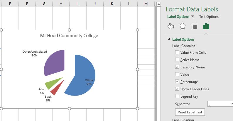
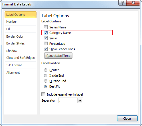
☝️How to Create a Pie Chart in Excel (Free Template) In the task pane that appears, do the following to spruce up your data labels: Navigate to the " Label Options " tab. Under " Label Options, " select " Category Name " to display the product categories next to the actual values. Under " Label Position, " click " Outside End " to push the labels outside the pie chart. Line Column Chart | Two Axes - QI Macros Excel Add-in Creating a Line Column Combination Chart in Excel . You can create a combination chart in Excel but its cumbersome and takes several steps. Select your data and then click on the Insert Tab, Column Chart, 2-D Column. Note: Make sure your labels are formatted as text or they will be added to the chart as a third set of bars. Next, right click on ... How To Make A Pie Chart - PieProNation.com 1. Create your columns and/or rows of data. Feel free to label each column of data excel will use those labels as titles for your pie chart. Then, highlight the data you want to display in pie chart form. 2. Now, click "Insert" and then click on the "Pie" logo at the top of excel. 3.
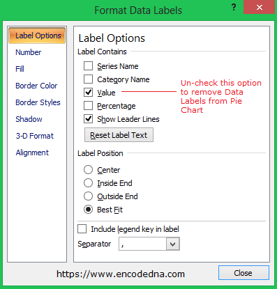
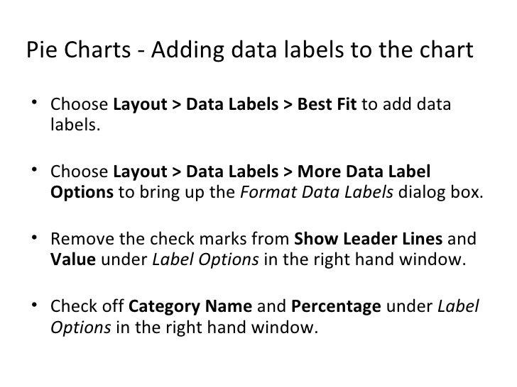
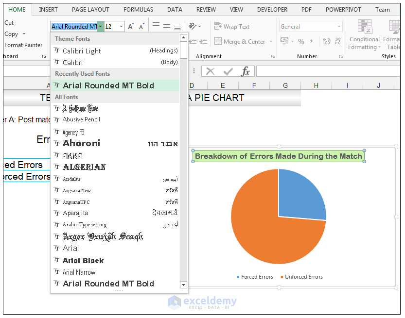
How to add data labels to a pie chart in excel. Add a pie chart - support.microsoft.com To switch to one of these pie charts, click the chart, and then on the Chart Tools Design tab, click Change Chart Type. When the Change Chart Type gallery opens, pick the one you want. See Also. Select data for a chart in Excel. Create a chart in Excel. Add a chart to your document in Word. Add a chart to your PowerPoint presentation How to Make a Pie Chart in Excel & Add Rich Data Labels to ... Formatting the Data Labels of the Pie Chart 1) In cell A11, type the following text, Main reason for unforced errors, and give the cell a light blue fill and a black border. 2) In cell A12, type the text Sinusitis, and give the cell a black border, and align the text to the center position. How to Make a Pie Chart in Excel (Only Guide You Need ... To add labels to the slices of the pie chart do the following. 1 st select the pie chart and press on to the "+" shaped button which is actually the Chart Elements option Then put a tick mark on the Data Labels You will see that the data labels are inserted into the slices of your pie chart. excel - How to not display labels in pie chart that are 0% ... I have some data in excel that I want to graph in a pie chart (see image 1) where the text will be the labels and the numbers will turn into percentages. The problem is, when i go to graph the data, it shows the labels for ALL of the sections, even the ones that are 0% in the pie chart. So this really overtakes my entire chart.
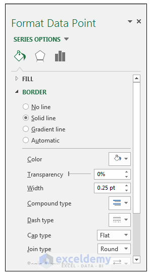
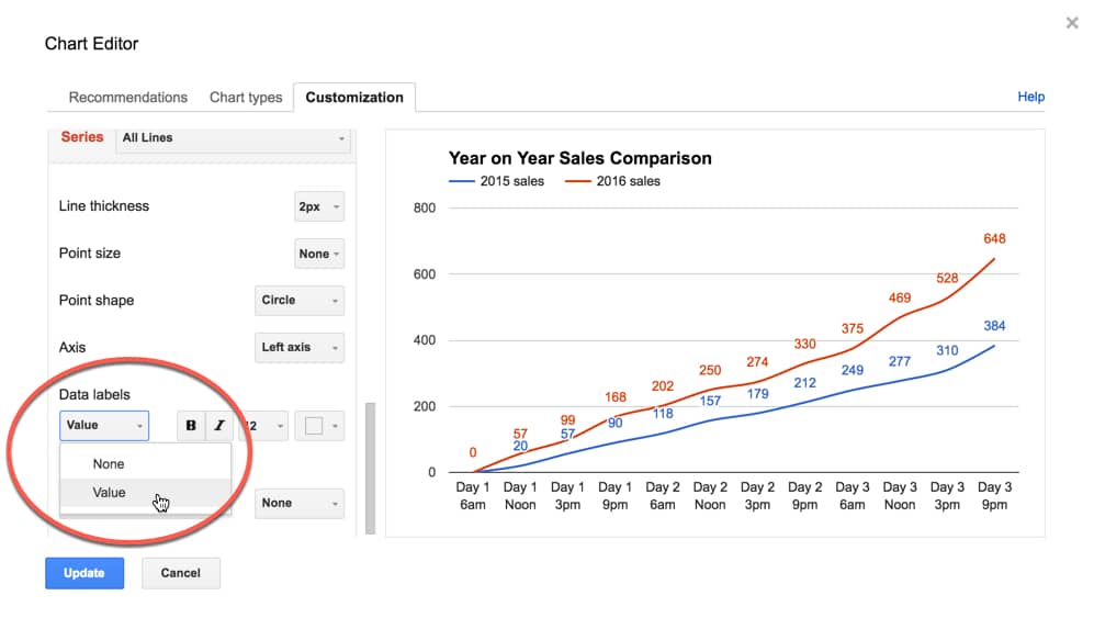
How to make a pie chart in Excel - EvalCentral Blog You do this by right clicking on the pie chart and selecting "Add Data Labels" from the menu. Changing the Label Position The labels need more work. I don't like Excel's "Best Fit" so I'm going to change the label position. Just right click on the label and select "Format Data Labels" to bring up the menu. Adding the Category Name to the Data Label Chart.ApplyDataLabels method (Excel) | Microsoft Docs For the Chart and Series objects, True if the series has leader lines. Pass a Boolean value to enable or disable the series name for the data label. Pass a Boolean value to enable or disable the category name for the data label. Pass a Boolean value to enable or disable the value for the data label. How to add a line in Excel graph: average line, benchmark ... 12/09/2018 · Right-click the selected data point and pick Add Data Label in the context menu: The label will appear at the end of the line giving more information to your chart viewers: Add a text label for the line. To improve your graph further, you may wish to add a text label to the line to indicate what it actually is. Here are the steps for this set up: Pie Chart in Excel - Inserting, Formatting, Filtering ... To add Data Labels, Click on the + icon on the top right corner of the chart and mark the data label checkbox. You can also unmark the legends as we will add legend keys in the data labels. We can also format these data labels to show both percentage contribution and legend:- Right click on the Data Labels on the chart.
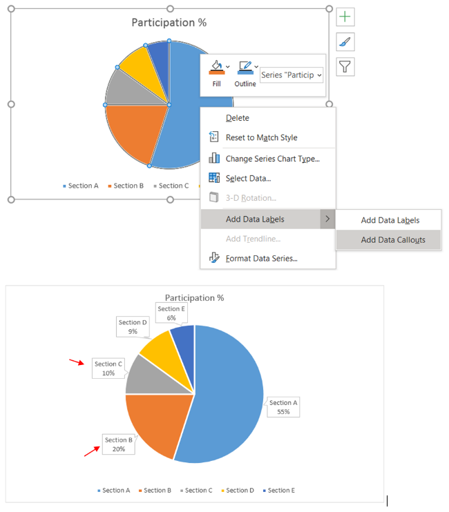
How to Create Pie of Pie Chart in Excel? - GeeksforGeeks Creating Pie of Pie Chart in Excel: Follow the below steps to create a Pie of Pie chart: 1. In Excel, Click on the Insert tab. 2. Click on the drop-down menu of the pie chart from the list of the charts. 3. Now, select Pie of Pie from that list. Below is the Sales Data were taken as reference for creating Pie of Pie Chart: python - Customize data labels in pandas pie chart - Stack ... I am trying to create a python pie chart from a dataframe with customized data labels. The dataframe that I am working off of contains percentages the correspond to each of the pie chart sections. I would like to display those percentages as data labels rather than the percent values of the totals of the whole. Excel does allow me to do that. Display data point labels outside a pie chart in a ... Create a pie chart and display the data labels. Open the Properties pane. On the design surface, click on the pie itself to display the Category properties in the Properties pane. Expand the CustomAttributes node. A list of attributes for the pie chart is displayed. Set the PieLabelStyle property to Outside. Set the PieLineColor property to Black. Add or remove data labels in a chart - support.microsoft.com For example, in the pie chart below, without the data labels it would be difficult to tell that coffee was 38% of total sales. Depending on what you want to highlight on a chart, you can add labels to one series, all the series (the whole chart), or one data point. Add data labels. You can add data labels to show the data point values from the ...
How to Create a Pie Chart in Excel using Worksheet Data
How to Make a Pie Chart in Excel 2013 - Solve Your Tech Step 4: Click the Pie Chart button in the Charts section of the ribbon, then choose the pie chart style you want to add to your spreadsheet.. Note that this Charts group in the ribbon has a variety of other types of charts or graphs that you could create instead. If a pie chart isn't what you need then you can simply click a different chart type and see if it provides the visual data layout ...
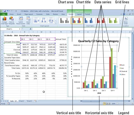
Getting to Know the Parts of an Excel 2010 Chart - dummies
38 excel chart move data labels How to Create a Bar Chart With Labels Above Bars in Excel In the chart, right-click the Series "Dummy" Data Labels and then, on the short-cut menu, click Format Data Labels. 15. In the Format Data Labels pane, under Label Options selected, set the Label Position to Inside End.
How to Make a Pie Chart in Excel & Add Rich Data Labels to The Chart!
How to plot a pie chart in Excel | Basic Excel Tutorial Next, click the icons next to the chart to add any other finishing touches. Here are some of the adjustments and customizations to add. You can format your pie chart's axis title or data labels. Here click on the Chart Elements icon on the right side of your chart. It is represented by a plus sign icon.
Charts in excel 2007
How to Make a Pie Chart in Excel - WinBuzzer Click on your pie chart in Excel and choose a style from the "Chart Design" tab You'll find various styles above the "Chart Styles" heading which will give your chart a fresh look. Press "Change...

Breaking down hierarchical data with Treemap and Sunburst charts - Microsoft 365 Blog
Show data in a line, pie, or bar chart in canvas apps ... 15/02/2022 · The import control is used to import Excel-like data and create the collection. The import control imports data when you are creating your app, and previewing your app. Currently, the import control does not import data when you publish your app. Press Esc to return to the default workspace. Add a pie chart. On the Insert tab, select Charts, and then select Pie …

Creating a Pie Chart in Excel
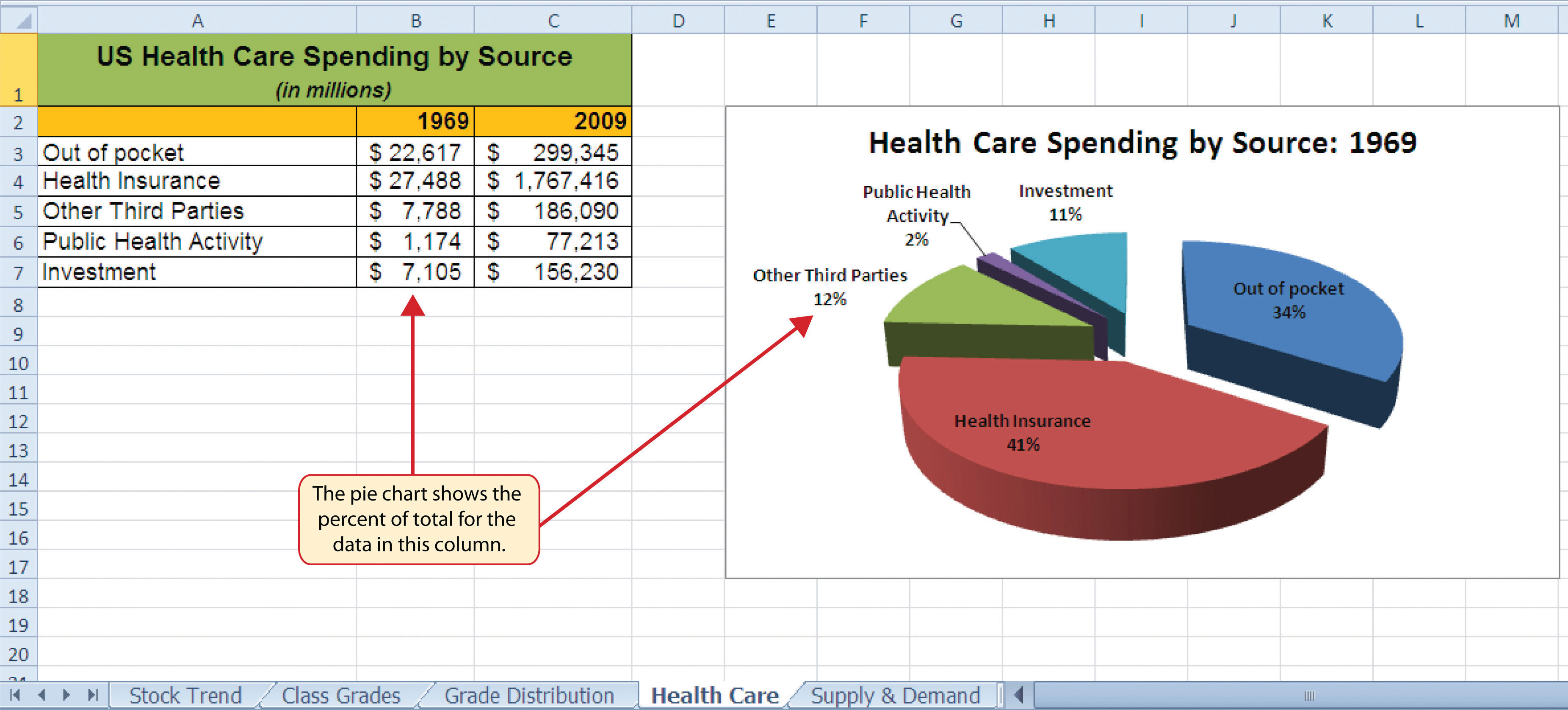
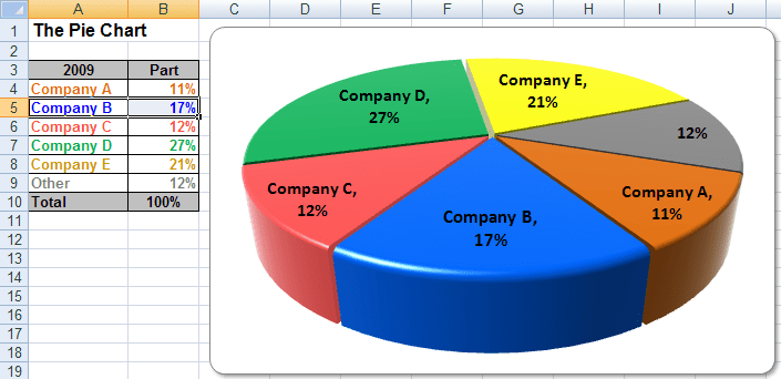
Add Percentage To Pie Chart In Excel - foxmob863.netlify.app You can add data labels to show the data point values from the Excel sheet in the chart. This step applies to Word for Mac only: On the View menu, click Print Layout. If you want to create a pie chart that shows your company (in this example - Company A ) in the greatestpositive light:
ExcelSirJi | Excel Data Tips | How to Create Pie Chart in Excel (Complete Tutorial) ExcelSirJi
How to Show Percentage in Pie Chart in Excel? - GeeksforGeeks The steps are as follows : Select the pie chart. Right-click on it. A pop-down menu will appear. Click on the Format Data Labels option. The Format Data Labels dialog box will appear. In this dialog box check the "Percentage" button and uncheck the Value button. This will replace the data labels in pie chart from values to percentage.

How to Create a Pie Chart in Excel | Smartsheet
How To Make The Number Appear On Pie Chart Power Point ... How do I label a pie chart in Excel? To add data labels to a pie chart: Select the plot area of the pie chart. Right-click the chart. Select Add Data Labels. Select Add Data Labels. In this example, the sales for each cookie is added to the slices of the pie chart. Can you format numbers in PowerPoint?
How to Create Excel Pie Charts & Add Rich Data Labels to The Chart!
How to Create Bar of Pie Chart in Excel Tutorial! Step 9: while still on the label options in your Excel sidebar, click on the label position category to customize the data labels. Here you can decide the position or alignment of the data labels. For example, if you check 'outside end' on the checklist option, the data label will appear outside the pie chart.
4.1 Choosing a Chart Type – Excel For Decision Making
How to Create A 3-D Pie Chart in Excel [FREE TEMPLATE] Right-click on your 3-D pie graph and click " Add Data Labels. " Go to the Label Options tab. Check the " Category Name " box to display the names of the categories along with the actual market share data. Recolor the Slices Next stop: changing the color of the slices.Double-click on the slice you want to recolor and select " Format Data Point. "
Adding Percentages To Pie Chart In Excel - Chart Walls
8 Types of Excel Charts and Graphs and When to Use Them In this article, you'll learn about the many types of charts available to you in Microsoft Excel using examples from publicly available data provided by data.gov. The data set is drawn from the 2010 US Census; we'll use this data to show you how impressive it is when you pick the right Excel chart types for your data.
How can I annotate data points in Google Sheets charts? - Ben Collins
How to Create a Pie Chart in Seaborn - Statology How to Create a Pie Chart in Seaborn. The Python data visualization library Seaborn doesn't have a default function to create pie charts, but you can use the following syntax in Matplotlib to create a pie chart and add a Seaborn color palette: import matplotlib.pyplot as plt import seaborn as sns #define data data = [value1, value2, value3 ...
Excel 3-D Pie Charts
How To Make A Pie Chart With Percentages - PieProNation.com Creating A Bar Of Pie Chart In Excel. Just like the Pie of Pie chart, you can also create a Bar of Pie chart. In this type, the only difference is that instead of the second Pie chart, there is a bar chart. Here are the steps to create a Pie of Pie chart: Select the entire data set. In the Charts group, click on the Insert Pie or Doughnut Chart ...

How to Show Percentage in Pie Chart in Excel? - GeeksforGeeks
How to add a total to a stacked column or bar chart in ... 07/09/2017 · Add data labels to the total segment at the Inside Base position so they are at the far left side of the segment. Using the default horizontal axis you will …
Excel 3-D Pie charts - Microsoft Excel 2010
How to show all detailed data labels of pie chart - Power BI 1.I have entered some sample data to test for your problem like the picture below and create a Donut chart visual and add the related columns and switch on the "Detail labels" function. 2.Format the Label position from "Outside" to "Inside" and switch on the "Overflow Text" function, now you can see all the data label. Regards ...
How to Make a Pie Chart in Excel & Add Rich Data Labels to The Chart!
Create Pie Chart In Excel - PieProNation.com Please do as follows to create a pie chart and show percentage in the pie slices. 1. Select the data you will create a pie chart based on, click Insert > I nsert Pie or Doughnut Chart > Pie. See screenshot: 2. Then a pie chart is created. Right click the pie chart and select Add Data Labels from the context menu. 3.
Pie Chart Examples | Types of Pie Charts in Excel with Examples
How To Make A Pie Chart - PieProNation.com 1. Create your columns and/or rows of data. Feel free to label each column of data excel will use those labels as titles for your pie chart. Then, highlight the data you want to display in pie chart form. 2. Now, click "Insert" and then click on the "Pie" logo at the top of excel. 3.
Post a Comment for "40 how to add data labels to a pie chart in excel"